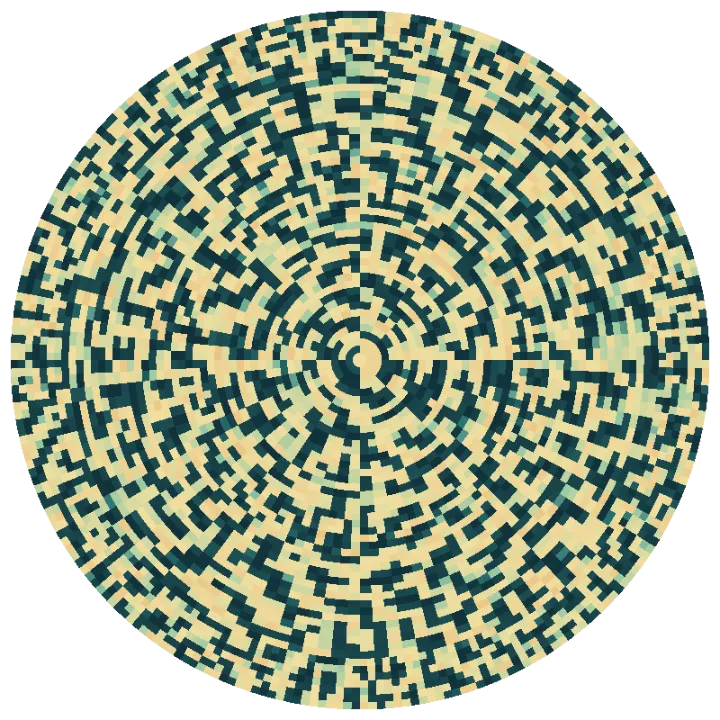
Animals in a forest are never spread evenly. Deer crowd one valley and skip the next. We usually credit the landscape: more food here, more cover there.
The map above has no better places. Every cell is identical, and the patches appeared anyway. Where do they come from?
Where this starts
How does a leopard get its spots?
In 1952 Alan Turing asked how a nearly uniform ball of cells ends up with spots and stripes.1
Two chemicals spread through the skin. An activator makes more of itself. An inhibitor suppresses it and spreads faster. Each patch of activator switches itself on and, through the inhibitor, switches off a ring around it: a spot. Change the rates and you get stripes. Nothing decides where the spots go.
Here prey are the activator and predators, who roam further, the inhibitor. The skin is a forest maze. Does it still work?
Question 1
Why do numbers change if nothing moves?
Prey multiply. Predators eat them and multiply until the prey run out, then starve. The prey recover and it repeats.
Rates
Lotka–Volterra with limited resources and, for cycling, saturating feeding. Both start at prey 10, predators 3. The vertical axis rescales.
Question 2
What happens when animals move?
On average they drift from crowded places to empty ones.
Here nothing is born or dies, so only movement is left. Six patches of forest joined by trails, sixty animals in the first. Close the middle trail and see what happens.
Setup
Six equal habitats, initial population [60, 0, 0, 0, 0, 0], diffusion 0.8. Paired exchanges conserve the total. This network of cells and passages is a graph.
Question 3
Why don’t all places cycle in step?
Because booms spread. Prey spill into the next corridor and predators follow. The boom travels as a wave, so neighbouring places sit at different points in the cycle.
Rates
r = 0.6, K = 100, a = 0.12, h = 0.5, e = 0.3, m = 0.3, c = 0; Dᵤ = 1.5, Dᵥ = 0.08. Seed 11, depth-first maze, 1,200 creatures in patches. Circular size 22, honeycomb 20, square 48, hexagonal 14 — shapes differ in cell count too, so this is not a shape-only comparison.
Question 4
Can a pattern stay put?
Yes, if predators range further than prey and suffer when crowded. A surplus of prey feeds predators that spread out and thin the prey around it. Small differences grow instead of fading: a spot, in a forest.1
Three identical mazes, same starting noise. Only the roaming differs.
Predators roam
Everyone roams alike
No one roams
Rates
r = 0.6, K = 100, a = 0.12, h = 0.5, e = 0.3, m = c = 0.03. Left: Dᵤ = 0.03, Dᵥ adjustable. Middle: both 0.03. Right: both 0. Same 8 × 8 depth-first maze, seed 11, starting at the coexistence balance ±1%. Runs stop at t = 240. Patchiness is the standard deviation of prey across cells. Predator crowding (c) is an extra rule; without it these equations cannot form a Turing pattern.
Question 5
Is it fragile?
No. Once the first maze settles, tap a cell to add twenty prey. The patch bulges, then heals.
Knocked in one cell or three, it returns to match the untouched run (correlation 0.995).
Question 6
Does the landscape’s shape matter?
It decides which patterns are possible. A maze can vary only in certain ways, its modes, from broad swells to cell-by-cell flicker. Each dot is one of this maze’s 64. Dots above the line grow.2
So what?
Patches aren’t always about the land.
An even world with a predator–prey cycle, movement, and predators that roam further will form its own patches, and restore them when disturbed.
Close a trail and the patches change. A road through a forest does that.
The equations
dvᵢ/dt = e F(uᵢ)vᵢ − m vᵢ − c vᵢ² + Dᵥ Σⱼ(vⱼ − vᵢ)
F(u) = a u / (1 + a h u)
u: prey; v: predators. r growth, K capacity, a attack, h feeding time, e conversion, m mortality, c crowding, D diffusion (“roaming”). Sums run over open neighbours only; walls allow no flow. Every cell has equal capacity whatever its drawn size.
Graph Laplacian L = degree − adjacency. The growth curve in question 6 is the largest real eigenvalue of J − λ diag(Dᵤ, Dᵥ), where J is the reaction Jacobian at the balance point.
Numerics, colour & limits
Live figures use an adaptive, positivity-preserving second-order solver, pause when offscreen and replay exactly from their seed. The stability check in question 5 ran the same solver to t = 240, added 20 prey to one or three cells, ran on to t = 400 and compared prey across all 64 cells with an untouched run.
The opening map replays a real recording, not a live run (the rates of question 4 with Dᵥ = 3; depth-first mazes, seed 11; circular 48, honeycomb 40, square 80, hexagonal 32; t = 0–180 every 2, interpolated). Its colour is prey density 0–65, clipped above, stored at 1/255 of that range. Live mazes blend prey/100 and predators/30 after square-root scaling; brightness follows total density.
A numerical demonstration, not an ecological forecast. Outcomes depend on rates, maze, seed and resolution. The “in the wild” notes are analogies to published observations, not claims that these equations describe those systems.
Credits & sources
Built by Samhan with GPT-6 Astra. Maze code and the Turing-pattern idea: Raziman T. V. (@razimantv). MIT licence.
- A. M. Turing (1952). The chemical basis of morphogenesis.
- H. Nakao & A. S. Mikhailov (2010). Turing patterns in network-organized activator–inhibitor systems.
- C. Elton & M. Nicholson (1942). The ten-year cycle in numbers of the lynx in Canada. Journal of Animal Ecology 11.
- O. N. Bjørnstad, M. Peltonen, A. M. Liebhold & W. Baltensweiler (2002). Waves of larch budmoth outbreaks in the European Alps. Science 298.
- M. Rietkerk & J. van de Koppel (2008). Regular pattern formation in real ecosystems. Trends in Ecology & Evolution 23.
- S. Kondo & R. Asai (1995). A reaction–diffusion wave on the skin of the marine angelfish Pomacanthus. Nature 376.